• Impact attribution of categorical dimensions on univariate variables
  • QUESTION
    • EXAMPLE USE CASE
  • SCENARIO 1: PLT
    • METHOD
  • SCENARIO 2: SITE TRAFFIC
    • METHOD
  • SCENARIO 3: CHANGE IN PLT
    • METHOD
  • READING THE RESULTS
  • CONCLUSION & CAVEATS
  • CHANGELOG

Impact attribution of categorical dimensions on univariate variables

QUESTION

“I have tabular data constructed from samples with multiple categorical dimensions, how do I explain each category’s contribution to the AVG or SUM”

“I have panel data that is an aggregate of multiple rows over time, how do I figure out which of the constituent rows is causing an observed change in the aggregate?”

EXAMPLE USE CASE

Let’s expand the question with a concrete example. An easy and common goal that people have is understanding their website traffic. In this example, we want to determine what is going on when there is a significant change in website traffic. As in: what circumstances are leading to the change in traffic.

Assume we have raw samples of data in the schema:

{
  // Categorical
  route: "/home",
  country: "US",
  region: "CA",
  device: "desktop",
  browser: "firefox",
  cluster: "clust05",
  host: "host19992",

  // Integers
  timestamp: +new Date(),
  page_load_time: 1200, // ms
}

Each sample in our dataset will represent one page visit and contains information from the server that generated the page and the client that is visiting the page.

We will use a variation of permutation testing and marginal effects analysis to help us determine 1) the impact each categorical dimension has on the global aggregate and 2) the impact that the change in each dimension has on the global aggregate.

While they are very similar sounding, the 1st is analyzing only data from within a given time period, while the 2nd is analyzing data from two time periods

For our scenarios, we will be using country as the dimension we are choosing to analyze, but in practice, one could and would analyze each of the dimensions to determine which are relevant to the situation

SCENARIO 1: PLT

We want to understand how each country is affecting the global page load time

METHOD

To determine each country’s impact on the actual average PLT (page load time) of the website, we will iterate through each country and estimate the global average PLT and the global COUNT with that country excluded from the data. We then compare the estimated values against their real values to determine the perceived change from the global aggregate that each row is providing. We refer to the perceived change as the row impact and will use it to figure out which rows are likely candidates for investigation.

First, we retrieve our data:

SELECT
  AVG(page_load_time), COUNT(1)
  FROM pagestats
  WHERE timestamp > TIME("-1 hour") and timestamp < NOW
  GROUP BY country

This query will return a table with each row representing the average page load time from each country and how many visits came from a country from the past hour.

Then we run our code:

rows = execute(<QUERY>);
real_sum = sum([row.page_load_time * row.count for row in rows])
real_count = sum([row.count for row in rows])
real_avg = real_sum / real_count
impacts = []

for row in rows:

    sum_without_row = real_sum - (row.page_load_time * row.count)
    count_without_row = real_count - row.count
    estimated_avg = sum_without_row / count_without_row
    estimated_delta = (estimated_avg - real_avg) / real_avg

    impacts.append((estimated_delta, row))

# sort the rows by absolute impact
impacts.sort(key=lambda tup: abs(tup[0]), reverse=True)

Now we have our rows sorted by absolute impact, where the impact is the measure of how much each row is affecting the global aggregate had that row been excluded from the data.

(See the section on reading results below for more details)

SCENARIO 2: SITE TRAFFIC

We see a dip in website traffic and want to understand which country (or countries) it is coming from.

METHOD

For calculating the impact that a country is having on website traffic (over time), we will use a technique similar to the previous one, but with two main differences: 1) we are only examining the COUNT (not AVG) because we are looking only at visits and 2) we will be using data from two time periods

Specifically - we will take the time period over where we see the dip and compare it to a relevant time period of the same length. For example, if we see a dip in the last hour, we can take the last hour of data and compare it against data from a day ago or a week ago of the same duration (1 hour) and ask what has changed.

Again, we start by taking one dimension (country) and examining the data to see if there are any leads.

SELECT
  COUNT(1)
  FROM pagestats
  WHERE timestamp > TIME("-1 hour") and timestamp < NOW
  GROUP BY country

SELECT
  COUNT(1)
  FROM pagestats
  WHERE timestamp > TIME("-25 hours") and timestamp < TIME("-24 hours")
  GROUP BY country

For each row, instead of removing the data from the current COUNT, we will substitute the previous value for each row and calculate what the COUNT would have been had this row remained unchanged

rows_now = execute(<QUERY 1>)
rows_prior = execute(<QUERY 2>)

real_count = sum([row.count for row in rows_now])
impacts = []

for row_now in rows_now:
    row_prior = get_prior_row(row_now, rows_prior)

    # subtract the current row value and add in the old value, so we can
    # pretend like the row never changed - the new sum will tell us what
    # effect the change in the rest of the traffic would have had without
    # this row
    count_with_old_row = real_count - row_now.count + row_prior.count
    estimated_delta = (real_count - count_with_old_row) / real_count
    impacts.append((estimated_delta, row))

# sort the rows by absolute impact
impacts.sort(key=lambda tup: abs(tup[0]), reverse=True)

SCENARIO 3: CHANGE IN PLT

We see an increase in our page load time and want to understand where it is coming from

METHOD

This is similar to SCENARIO 2, but we will also take into account the AVG page load time

By this point, the queries and code should look familiar:

SELECT
  COUNT(1), AVG(page_load_time)
  FROM pagestats
  WHERE timestamp > TIME("-25 hours") and timestamp < TIME("-24 hours")
  GROUP BY country

SELECT
  COUNT(1), AVG(page_load_time)
  FROM pagestats
  WHERE timestamp > TIME("-25 hours") and timestamp < TIME("-24 hours")
  GROUP BY country

rows_now = execute(<QUERY 1>)
rows_prior = execute(<QUERY 2>)

real_sum = sum([row.page_load_time * row.count for row in rows_now])
real_count = sum([row.count for row in rows_now])
real_avg = real_sum / real_count
impacts = []

for row_now in rows_now:
    row_prior = get_prior_row(row_now, rows_prior)

    # subtract the current row value and add in the old value, so we can
    # pretend like the row never changed - the new sum will tell us what
    # effect the change in the rest of the traffic would have had without
    # this row
    count_with_old_row = real_count - row_now.count + row_prior.count
    sum_without_row = real_sum - (row_now.count * row_now.page_load_time)
    sum_with_old_row = sum_without_row + row_prior.page_load_time

    estimated_avg = sum_with_old_row / count_with_old_row
    estimated_delta = (real_avg - estimated_avg) / real_avg

    impacts.append((estimated_delta, row))

# sort the rows by absolute impact
impacts.sort(key=lambda tup: abs(tup[0]), reverse=True)

READING THE RESULTS

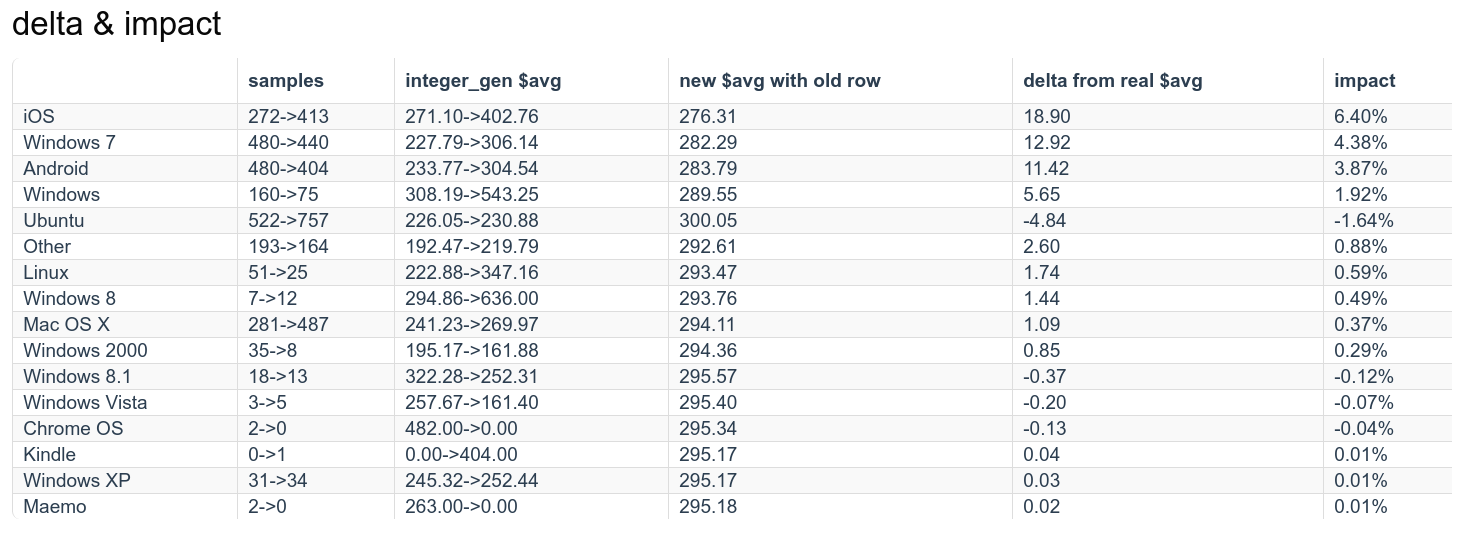
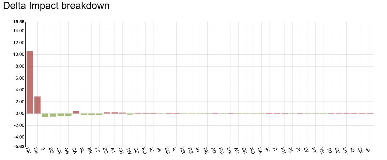
For each of the above scenarios, an estimated impact is computed for each row and normalized against the real_avg or real_count to give a measure (aka the impact) of how much that row is affecting the global aggregates

The higher the absolute value of the impact, the more effect that row has had on the global aggregates. The sign of the impact indicates which direction the row is pulling the aggregate.

Using impact as a ranking of which rows are affecting the global (and by how much) is useful, but we can further break down why each row is affecting the global aggregate.

When we are using two time periods (Scenarios 2 and 3), notice that the possible outcomes for any row are:

• row count: raised or lowered
• row aggregate: raised or lowered
• impact: positive or negative

Determining the above values for each row lets us understand if the row is affecting the global aggregate through its change in value, through a change in presence (higher or lower row count) or a combination of both.

The most straight-forward situation is when a particular row’s value suddenly becomes more costly - maybe a particular page became more expensive to compute. Had all other rows remained unchanged, this would show up as a raise in the global average.

Alternatively, a row may have a lowered sample count (perhaps a new bug is manifesting during page generation), leading to a decrease in its presence inside the global population. If that row had a low aggregate, the end result would be that the global average raised, but the only thing that has changed was the row’s count.

Similarly, an increase in presence (due to uncontrolled XHR requests, f.e.) could account for a decrease in the global average if a low cost endpoint is being hit.

It’s important to note that in the above interpretations, the effect of any given row can be masked by changes in other rows. Impact analysis lets us examine how any row’s change is affecting the global, despite the change in other rows.

CONCLUSION & CAVEATS

Using the above methods, one can create estimates of how the values inside underlying distributions are shaping the global aggregates, giving insight into the makeup of a distribution in a single time period or the way a distribution has changed over two time periods.

This particular technique only works for aggregates that can be unrolled, such as AVG, SUM and COUNT. Percentile aggregates can not easily be merged / unmerged without a full histogram available.

CHANGELOG

2016-06-08

• clearer intro questions (lericson)

2016-06-06

• less headings, clearer text (lericson)
• more explanatory text (mads)

2016-06-01

• fix typographical mistakes in pseudocode
• add more detail to scenario 2’s method
• add mention of marginal effects to summary (wuch)

2016-05-31

• first write up of impact analysis