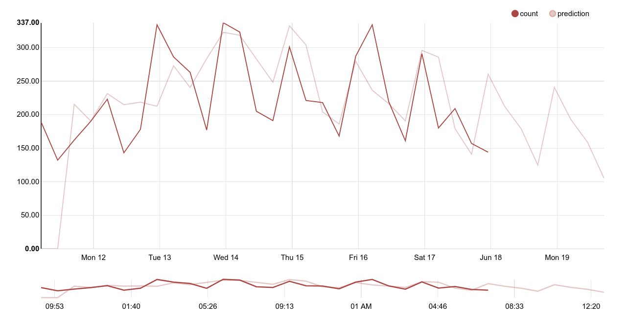
Time series forecasting with multi-seasonal exponential smoothing

Time series forecasting with multi-seasonal exponential smoothing

time series forecasting

In this page, we will go over implementation details for the multi-seasonal holt winters’ set of smoothing equations as referenced in

If you are unfamiliar with the original holt winters’ equations, you can see them here. The formulas alone are pretty unintuitive, so I recommend reading grisha’s guide

MOTIVATION

When examining time series related to human behavior, daily patterns emerge. If we spend enough time squinting at graphs (or just like to hypothesize), we might guess that not only is there a daily pattern, but there tends to be a weekly pattern, as well.

While there are many implementations of the single season holt-winters’ equations (which all coincidentally point to the NIST guide), there are not too many implementations of the multi-seasonal models - this page hopes to help others convert their models to multi-seasonal.

ORIGINAL EQUATIONS

Recall the original equations for the multiplicative model:

# overall smoothing:
S[t] = alpha * (Y[t] / I[t-L]) + (1 - alpha) * (S[t-1] + B[t-1])

# NOTE: B and beta are aligned in the below equations, but not in the original
# NIST equations which has gamma / B aligned and I / beta aligned,
# but B and beta make more sense to me

# trend smoothing:
B[t] = beta * (S[t] - S[t-1]) + (1 - beta) * B[t-1]

# seasonal smoothing
I[t] = gamma * (Y[t]/S[t]) + (1 - gamma) * I[t-L]

Easy, right?

UPDATING TO THE MULTI-SEASONAL MODEL

First, we re-define gamma, L and I and turn them into arrays of values, one value per season. (we are multi-seasonal, after all)

gamma = [G0, G1, ...]
L = [L0, L1, ...]
I = [I[L0], I[L1], ...]

The initialization of the second season is much simpler than the initialization of the first season. In the multiplicative model, we will initialize all the values to 1 (the multiplicative identity), since the seasonal co-efficients are multiplied together when making our forecasts.

for i in xrange(len(I)):
  for j in xrange(len(L[i])):
    if i > 0:
      I[i][j] = 1

When updating parameters, we consider the first season to be the predictor of behavior and the second season captures the difference in the expected behavior of the first season and the actual outcome. In other words, we consider the second season to be “correcting” the errors of the first by capturing its residuals.

In equation form:

S[t] = alpha * (Y[t] / I[0][t-L0] / I[1][t-L1]) + (1 - alpha) * (S[t-1] + B[t-1])
I[0][t] = gamma[0] * (Y[t] / S[t] / I[1][t-L1]) + (1 - gamma[0]) * (I[0][t-L0])
I[1][t] = gamma[0] * (Y[t] / S[t] / I[0][t-L0]) + (1 - gamma[0]) * (I[1][t-L1])

Wow… what a mouthful. Instead of hardcoding indeces, let us rewrite this more clearly. With a loop, we calculate the overall product of the seasonal co-efficients and then subtract out each season to find the residual factors.

# calculate seasonal co-efficient
prod_seasons = 1
for i in xrange(len(I)):
  prod_seasons *= I[i][t-L[i]]

# update our smoothed average
S[t] = alpha * (Y[t] / prod_seasons) + (1 - alpha) * (S[t-1] + B[t-1])

# update our seasonal models
for i in xrange(len(I)):
  residuals = prod_seasons / I[i][t-L[i]]
  I[i][t] = gamma[i] * (Y[t] / S[t] / residuals) + (1 - gamma[i]) * (I[i][t-L[i])

The forecasting procedure is similar to the single seasonal normal equations. The main difference is that we accumulate all our seasonal co-efficients before making the forecast.

prod_seasons = 1
for i in xrange(len(I)):
  prod_seasons *= I[i][t-L[i]]

forecast = (S[t] + m*B[t]) * prod_seasons

return forecast

And there we have it: multi-seasonal exponential smoothing.

If you were able to use the above to update your model, congratulations! If not, get in touch and let’s debug it together. Happy forecasting!

IMPLEMENTATION

Snorkel’s implementation of HW exp smoothing + a simple solver is available on github

CHANGELOG

2019-03-31

update github source link to port to snorkel-lite branch

2017-06-19

add a picture

2016-08-30

first write up of multi-seasonal exponential smoothing

log(v)